Reading Peter Muller

More than meets the eye

The year 2001 saw the birth of Quantitative Finance, a journal at the boundary between academia and practice. The lead paper in the very first issue was an “opinion paper” by a practitioner: “Proprietary Trading: Truth and Fiction.” It was three pages long and even included a photo of the smiling author.
Peter Muller never wrote—or said—anything as informative in the twenty-five years that followed. A recent video, for example, is basically a puff piece. To Muller’s credit, some of his songs tackle genuinely original topics, like the one he once wrote about a divorced billionaire. Maybe he lost interest in sharing ideas. Maybe he regretted putting something this informative into public view. Nobody knows.

Let’s go back to that opinion paper. I’m going to do a close reading and comment on bits that I find interesting. I hope you will stay for the ride. Most of this applies to both systematic and discretionary investing; less so to pure execution/flow strategies (merger arb, delta-one, index rebalancing).

Information Leakage

Let’s start at the end (emphasis mine):

My aim in this article was to be informative (and occasionally entertaining) while not telling you anything that my competitors or potential competitors would find useful. Unfortunately, the mere knowledge that it is possible to beat the market consistently may increase competition and make our type of trading more difficult. So why did I write this article? Well, one of the editors is a friend of mine and asked nicely. Plus, chances are you won’t believe everything I’m telling you. And if you do, well, I’ve always liked a challenge.

I know of another hedge fund manager who, many years ago, met with an expert in convertible arbitrage. The expert didn’t say much, but apparently hinted at capacity. In the (apocryphal) retelling, the expert was asked whether there would be a follow-up meeting. The manager replied: “Thanks—I know all I need to know.”

Just knowing that you can make, say, $1B a year in a strategy is extremely valuable information. Before Jane Street started generating profits in the tens of billions, other prop firms didn’t think it was possible. But it was. And now a few firms (Hudson River Trading, Citadel Securities) have made “very large” the new baseline. The next target becomes even larger, precisely because someone has demonstrated that it can be done.

There’s an analogue in mathematics: knowing that a conjecture is true can change everything. If it can be proved, someone will try harder—and someone eventually will. A famous episode captures the vibe. Here’s the standard version, via Wikipedia:

During his study in 1939, Dantzig solved two unproven statistical theorems due to a misunderstanding. Near the beginning of a class, Professor Spława-Neyman wrote two problems on the blackboard. Dantzig arrived late and assumed that they were a homework assignment. According to Dantzig, they "seemed to be a little harder than usual", but a few days later he handed in completed solutions for both problems, still believing that they were an assignment that was overdue. Six weeks later, an excited Spława-Neyman eagerly told him that the "homework" problems he had solved were two of the most famous unsolved problems in statistics. He had prepared one of Dantzig's solutions for publication in a mathematical journal. This story began to spread and was used as a motivational lesson demonstrating the power of positive thinking. Over time, some facts were altered, but the basic story persisted in the form of an urban legend and as an introductory scene in the movie Good Will Hunting.

Another example: in the TV series “Plur1bus,” an alien intelligence takes over humans by replacing their personalities with those of the aliens. Only a handful of humans are immune. They’re benevolent, they won’t kill the protagonist, and they can’t lie. One day, the protagonist asks an alien whether the takeover can be reversed. The alien doesn’t answer. The lack of an answer reveals that a method exists.

This dynamic shows up in finance interviews all the time. If a candidate can’t answer a question—“What is your capacity?” “Why do you use high-frequency data for low-frequency strategies?”—then, depending on the context, they may already have answered it. The information game in finance begins even before the interview does.

Performance Evaluation

When we evaluate past performance, we also look at peak-to-trough drawdowns (a measure of the maximum drop between consecutive maximum and minimum values of return over the life of the strategy) as an additional risk variable. This can help pick up serial correlation in portfolio returns that the Sharpe Ratio doesn’t capture.

I’m not sure how much “serial correlation” you really detect during a drawdown window. I’m not even sure the concept is well-posed over, say, a ten-trading-day episode. In a genuine distress event, you shouldn’t assume there is a stable data-generating process. Extremal statistics like drawdowns have large standard errors even when returns are uncorrelated, and for heavy-tailed distributions the variance itself may not be finite.

My (debatable) view is that the most effective way to estimate worst-case losses is not to stare harder at historical backtests, but to understand exactly what inefficiency the strategy exploits—and then build conservative scenarios that stress-test that mechanism.

Investment strategies have fixed capacities. As I increase the money invested in a strategy, my expected transaction costs increase while my pre-transaction cost estimate of expected return stays constant. Figure 1 shows an example of this—once my marginal expected return, net of transaction costs, crosses zero, increased investment in a strategy only loses money.

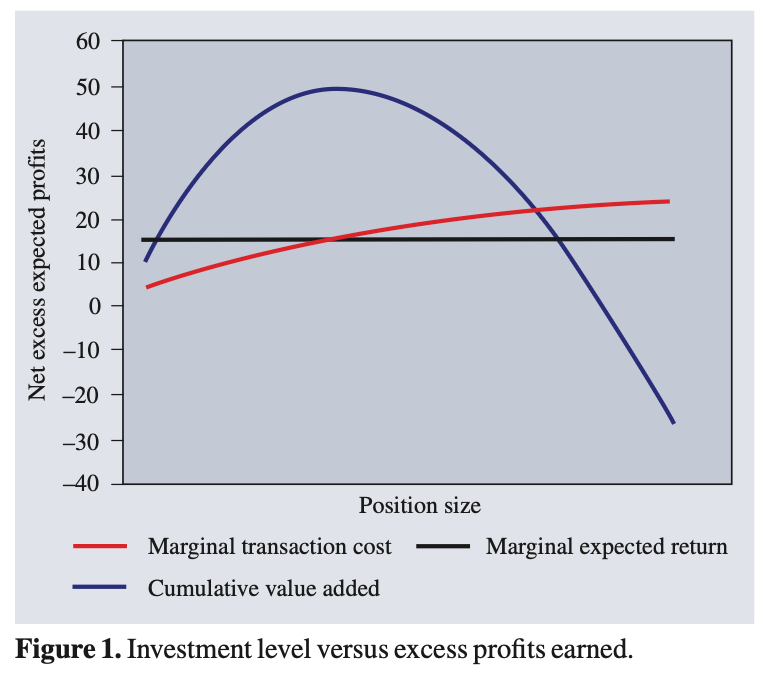
A small anecdote. Years ago I asked a portfolio manager, “Do you know what your trading costs were last year?” He said, “I think $5M?” The answer was closer to $75M.

Many (most?) portfolio managers—including systematic ones—are surprisingly insensitive to transaction costs. Fundamental PMs, especially, are perpetually hungry for volatility. But more volatility is not always better, and that’s Muller’s point.

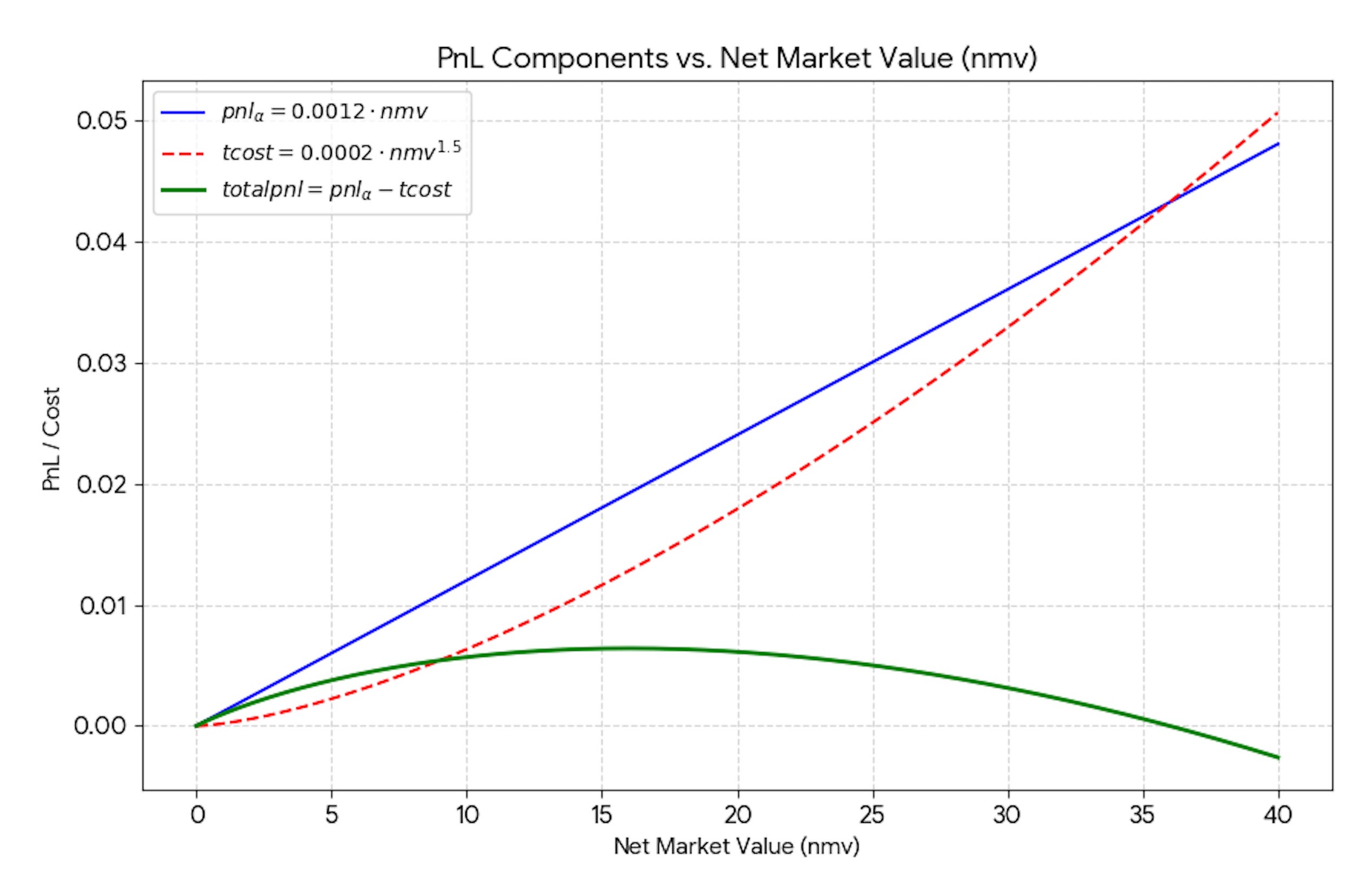
Here’s a toy version. Suppose NVIDIA is expected to gain 0.12% over the next two weeks. You must position for that date. Let www be the NMV you deploy in NVDA. Expected gross PnL (pre-costs) is 0.0012·w .Unit transaction costs are not linear. They are proportional to √w. These are not marginal costs. They are average costs. Let us make an example. You trade $20M. The costs are 0.0002*sqrt(20)*$20M = $17.9K. Unit costs are 0.0002 * sqrt(20) = 9bps. If you trade $40M, trading costs are 0.0002 * sqrt(40) * $40M = $50.6K. Unit costs are 0.0002*sqrt(40)=12.6bps. Both the first and the second $20M pay 12.6bps. The PnL reaches a maximum, and then decreases to the point that it becomes zero, or negative.

As a strategy develops, betting opportunities increase and returns for each bet increase. But a huge transaction-cost barrier must be overcome before a strategy becomes profitable. Once this is overcome, additional improvements will leverage profit much more efficiently than initial research will. Even though these improvements are harder to come by, the work is worth the effort.

This is an empirical statement, but it seems true to me. I have observed many instances of strategies that were profitable in backtests, that had good conceptual foundations, but could not “break through” because of execution limitations. These limitations can be latency-based, but not only. Being able to hide flow from your faster counterpart can be as important, or more. Operating in a firm that is well-suited to warehouse the risk of your trades or has positive flow externality can also be extremely important. Once these limitations are overcome, the next stage of profitability can be unlocked.

Incentives

Hedge fund managers are incentivized both by a percentage of the profits they make and by how much money they have under management. They are therefore less susceptible to the aforementioned agency issues, but not entirely free of them.

This hasn’t aged perfectly. Muller’s thesis is that asset managers are incentivized to gather assets without caring enough about performance because they earn a management fee on AUM. That’s mostly true, though competition has compressed fees and, in many segments, tracking error. The rise of passive management can be read as a market response to the asset-gatherers of yore.

What about hedge funds? Times have changed. Hedge-fund operating costs have grown over the past twenty-five years. Administration, technology, and talent are expensive, and many costs are roughly linear in scale. More AUM often means more limited partners—or fewer of them who require more attention. Larger organizations are more diversified, which in turn requires more bespoke technology and services. And talent has been repriced: searching for it is relentless and expensive, and paying for it is expensive too.

All of this is to say: the classic 2-and-20 model (2% management fee on AUM, 20% performance fee on net PnL above a high-water mark) is, in many cases, no longer adequate. A 2% fee doesn’t make anyone rich, and it often doesn’t even cover operating costs.

Platforms that pass costs through have been the big success story of the last two decades. But despite their size, the best platforms don’t treat “maximize AUM” as the primary goal. They are held to the standard of producing “equity-like returns with bond-like risk”: roughly 7–8% returns in excess of cash with low correlation to market benchmarks. Asset growth is, lexicographically, a distant second. By and large, successful hedge funds are capacity-constrained and manage their size to protect returns.

Performance

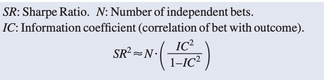
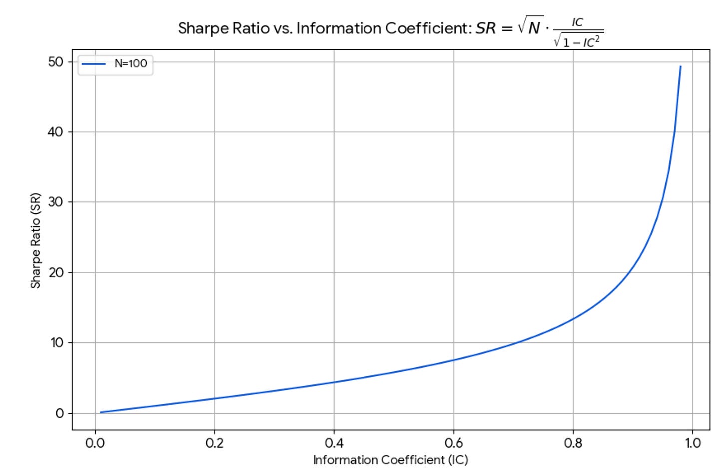
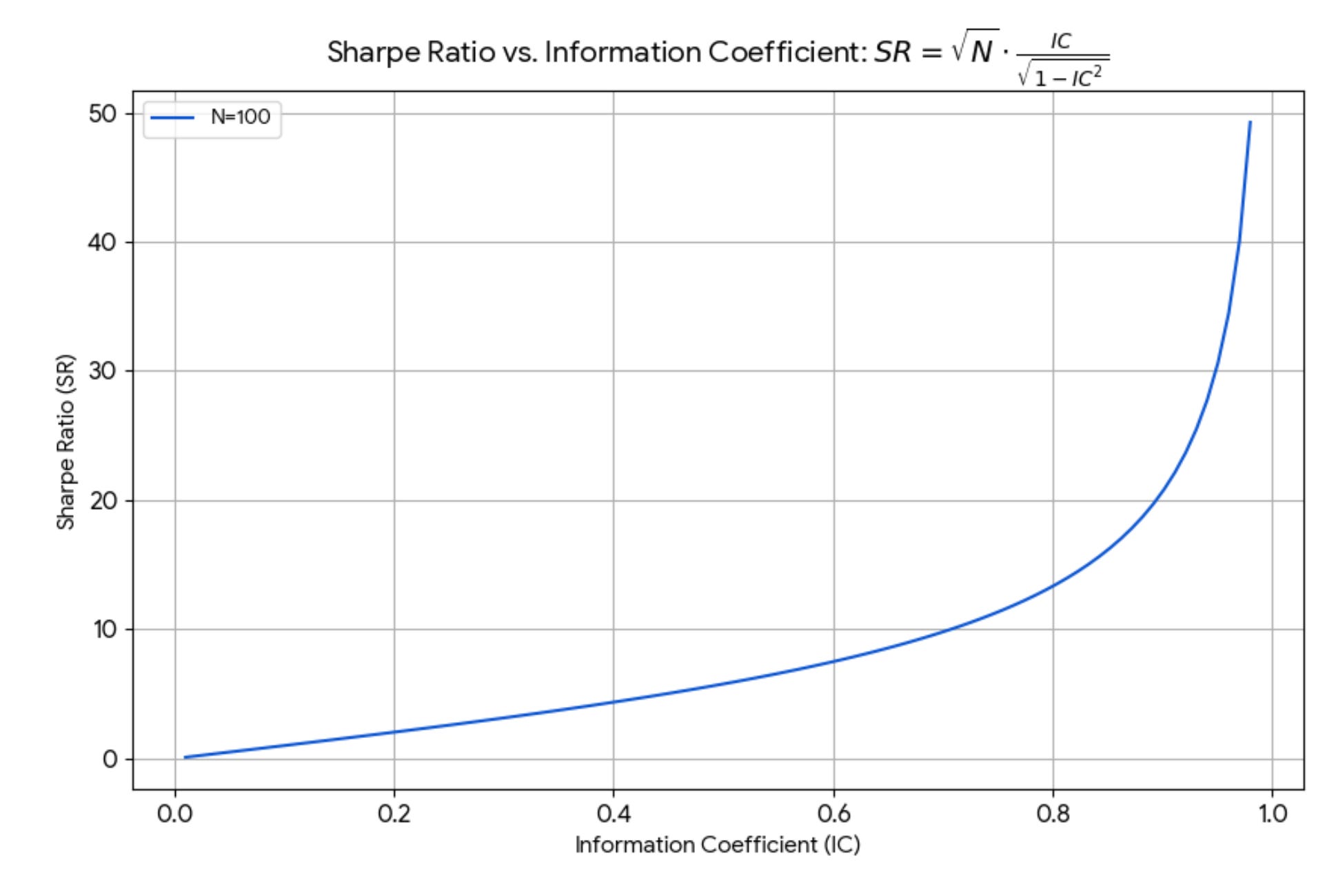
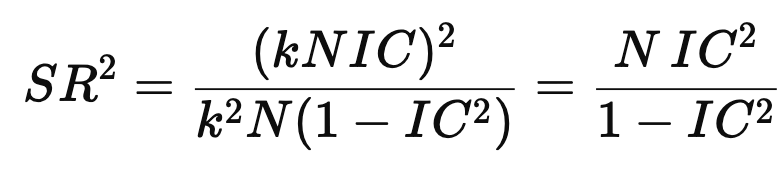
A strategy’s Sharpe Ratio is proportional to the number of independent bets taken by the strategy multiplied by the correlation of those bets with their outcome (figure 3). To get a higher SR, you need to increase the number of your bets or increase the strength of your forecasts.

This is an important formula. Active Portfolio Management had been out for only a few years in 2001 and wasn’t as widely known. The idea is still used constantly, usually in the shorthand

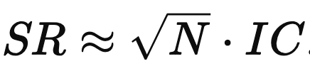
Muller’s expression is a slightly different—but equivalent—presentation. What does it mean?

1. There’s the usual sqrt(N)​ diversification effect: if you increase the number of assets while holding IC fixed, volatility scales like sqrt(N) while PnL scales like NNN. It’s a Central-Limit-Theorem-flavored fact of life.

2. If your cross-sectional forecasts are negatively correlated with cross-sectional returns (we are working in the cross section), you can still make money: flip the sign. Short yourself. You’ll profit—plus you’ll owe your therapist (or “performance coach,” i.e., a decaffeinated therapist for rich people) a large bill.

3. If IC were high, Sharpe would be enormous. With perfect foresight, you’d be infinitely rich with no risk. In real life, IC is tiny; IC = 0.01 is not large, so we’re in the linear regime.

4. For small IC (IC < 0.4, which is still very high!), the formula is linear and is well approximated by Grinold’s formula. For large IC, the Sharpe Ratio explodes. See the picture below.

   

I’d like to explain the formula in elementary terms. There’s a bit of algebra and probability, but nothing brain-damaging. Portfolio managers: you’re big boys and girls. You don’t have to read it—but your mom would be proud if you did.

Assume stock returns are uncorrelated. In the real world they aren’t, but you can remove a lot of correlation by subtracting common factor returns (the market factor and a petting zoo of additional factors). That process also makes the cross-sectional mean return (across stocks on a given day or minute) approximately zero: you’re now looking at idiosyncratic returns.

Also assume unit volatility. This isn’t true either, but you can z-score returns and reason in that space.

On a given period (days, minutes), you have standardized return predictions alpha(i) for stock i. Standardize those too, and assume they have cross-sectional mean zero. Write the relationship as

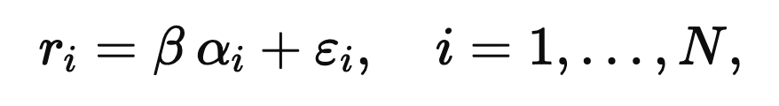
where epsilon(i) is noise with mean zero. In this standardized setup,

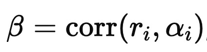
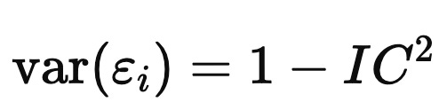
which ‘we call the Information Coefficient (IC). Taking cross-sectional variances gives

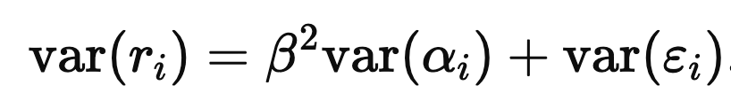
and since var(r_i) and var(α_i) are both one,

If you maximize expected PnL subject to a risk constraint, you obtain an optimal portfolio proportional to forecasts: w_i = kα_i​. The expected PnL is

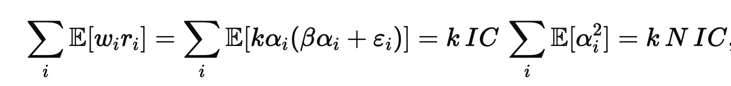
because E[α_i²]=1 under standardization and the noise term drops out.

For the risk, assume (for this toy derivation) that the α_iε_i terms are cross-sectionally independent with mean zero. Then

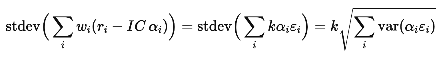
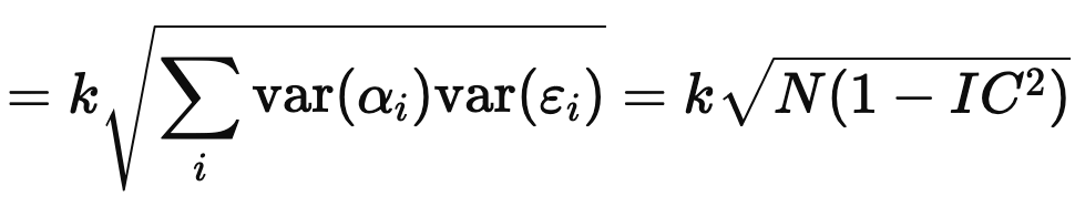
Therefore,

which is Muller’s (or Grinold & Kahn’s) formula.

In my opinion it is far better to refine an individual strategy by increasing both the number of bets within the strategy and the strength of the forecasts made in the strategy, than to attempt to put together lots of weaker strategies. Depth is more important than breadth for investment strategies.

[…]

I would much rather have a single strategy with an expected Sharpe Ratio of 2 than a strategy that has an expected Sharpe Ratio of 2.5 formed by putting together five supposedly uncorrelated strategies each with an expected Sharpe Ratio of 1. In the latter case you’re faced with the risk that the strategies are more correlated than you realize (think Long Term Capital). There is also the increased effort of ascertaining whether each individual strategy really has a Sharpe Ratio of 1.

These aren’t statements you can derive cleanly from first principles, and there isn’t universal agreement. But they’re interesting—and, in my opinion, mostly true.

To improve a business, there are two idealized approaches: depth-first and breadth-first.

Depth-first means refining an existing strategy. For example:

• Make more bets: extend the logic across markets, venues, and coverage.

• Add better inputs: new or higher-quality transactional data.

• Improve execution.

• Improve signal yield: use the same signal across horizons.

Breadth-first means combining distinct strategies. For example:

• Add discretionary credit to a set of high-frequency strategies.

• Add systematic futures to systematic equities.

• Add merger arb and delta-one to long/short equities.

• Add generalist long/short pods to a set of sector-focused PMs.

Muller’s advice is: go depth-first. Reasons:

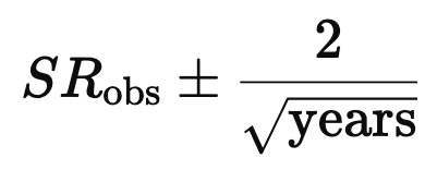
• Skill is easier to separate from luck when Sharpe is high. As a rough rule, a 95% two-sided confidence interval scales like

  

• Model risk is the possibility that the simplified mental model around which you have organized a business might be very wrong at times. Model risk takes many forms, usually one more form than the ones that you have imagined so far. Famously, the risk management framework of Long Term Capital Management was conceived primarily by Myron Scholes. And all the partners of LTCM were first-rate traders and finance intellectuals. What Muller says is (as I see it) that the first sign of intellectual humility is to be a hedgehog, not a fox. This statement might be the deepest and most important in his paper. The success of PDT is a testament to the approach.

On Investment Classification

Typically, shorter horizon strategies get their edge from providing temporal liquidity to a market place or predicting short-term trends that arise from inefficient trading. Longer-term models focus on asset pricing inefficiencies.

I find it useful to think about alpha as being a combination of three idealized mechanisms: information ("investing"), structure ("trading") and risk ("risk premia"). Something like this:

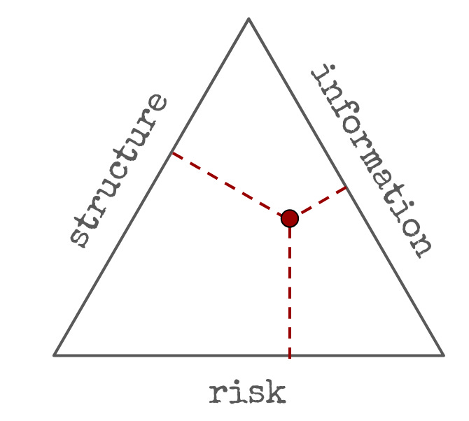
“Trading” profits arise mostly from structural inefficiencies, of which there are many. Some participants are institutionally required to trade at predetermined times, and in directions that intelligent participants can forecast. Other participants have funding costs and constraints that other participants can take advantage of. Certain participants have different risk appetite than others. These structural inefficiencies can arise from institutional constraints and physical limits, but even in an ideally designed market they would still exist because there are asymmetries among participants.

“Investing” profits arise mostly from informational inefficiencies. A portfolio manager reasons about the changes in the supply chain induced by AI and figures out that certain firms will benefit and others will suffer, before the information is priced by the market. Another portfolio manager remembers that an obscure tax exception for hotels is set to expire, and shorts them.

Lastly, “risk” consists of investing in known synthetic instruments (“factors”), in a way that is consistent with the risk tolerance of the participant. Bond/equity portfolios are an instance of it, and so is passive investing, and so is investing in “value” stocks, or “momentum”, or other styles.

These don’t exist in isolation; almost every real strategy mixes all three. Muller maps “trading” to structure and “investing” to a mix of risk premia and information—and he also associates investing with longer horizons:

Longer-horizon model-driven investment strategies have different issues. Since assets are held for longer periods of time, execution costs (although still important) are not the primary focus. Statistical inference becomes more difficult and the danger of overfitting or mining data becomes larger.

That may have been truer in 2001. Today, long/short discretionary equity often operates at an investment horizon close to slow stat arb. Execution costs are absolutely a primary focus.

Shorter-horizon investment strategies are desirable because they tend to create higher Sharpe ratios. If your average holding period is a day or a month, you have the opportunity of placing many more bets than if you hold positions for three months to a year or longer. On the flip side, shorter horizon strategies tend to have capacity issues (it’s easy to make a small amount of money with them, harder to make a lot of money).

The Sharpe formula we derived earlier is per “investment cycle” of length T. If there are 1/T investment cycles in one year, the the Sharpe Ratio is approximately equal to

(Sharpe Ratio Annualized)

= (Sharpe Ratio in a period) · sqrt(1/T)

≈ IC · sqrt(N/T)

Even if a systematic strategy has a lower IC than a discretionary one, it more than makes up for it by having a large investment universe N and a higher turnover 1/T. Can we quantify the capacity of a systematic strategy as a function of T? Not easy. A very rough estimate¹ suggests that, as long as the expected return of a trade depends on the investment horizon, and is increasing in T, the optimal capacity of the strategy is also increasing in T. So there is a trade-off between capacity and risk adjusted performance.

Risk Management

Risk management for longer-term strategies happens in portfolio construction: since rebalancing occurs less frequently, more care needs to be taken to ensure the portfolio is not exposed to unintended sources of risk.

[…]

Risk management for shorter horizon strategies tends to occur through position trading rather than portfolio construction. Assets are not held for long periods of time and portfolio characteristics change quickly. The biggest risk for shorter horizon strategies is model risk, or the risk that the trading strategy deployed has stopped working.

In its simplest form, the optimization problem looks like:

maximize total expected PnL
subject to risk ≤ max risk.

A more advanced version adds constraints:

maximize total expected PnL
subject to risk ≤ max risk and factor risk ≤ max factor risk.

The “subject to” part is what couples assets. Even if assets were uncorrelated you’d have a constrained problem. Correlations complicate it further—enough to keep people like me employed.

Much depends on operating at the risk boundary. You hit the boundary when (i) the firm has finite risk appetite and (ii) the strategy has enough capacity for constraints to bind. In higher-frequency strategies, capacity is often limited: transaction costs (impact, fees) eat into profitability. If the optimum lies in the interior (constraints slack), the objective becomes effectively separable: you can optimize assets more independently. The ongoing battle in high frequency is preventing capacity from collapsing below the economic threshold—and managing the “unknown unknowns” of model failure with safeguards designed for survival.

Conclusion

I don’t think there are three pages about investing that pack in more ideas than this one. PDT was a pioneering firm. Muller’s music may not be your cup of tea, but he is a more interesting writer than the vast majority of hedge fund managers.

1. The unit trading cost is proportional to sqrt(trade size) and is inversely proportional to the trading volume in the lifetime of the trade. The trading volume is v·T, where v is the number of shares traded per unit of time (say, hour). The total cost of of a trade is proportional to sqrt(trade size / T) · (trade size).
The expected return of a stock depends on the investment horizon; it’s reasonable to assume that it increases in T like T^ε for some positive exponent ε.The expected PnL is

[α· T^ε - constant · sqrt(trade size / T)]·(trade size)

We can optimize this function with. respect to trade size. The optimal trade size is proportional to α²T^1+2ε and the associated optimal PnL is proportional to α³T^1+3ε. There are (1/T) trades per stock in one year, and it follows that the PnL per year in a stock is proportional to α³T^3ε. As long as expected returns are increasing as a function of the investment cycle duration T, two facts emerge. First the optimal trading size decreases with T. Second, the optimal expected PnL of the strategy decreases with T.