
Information Coefficient, Transfer Coefficient And All That
[Originally Polemically Titled "The Transfer Coefficient Is Not What You Think It Is"]

“TC” is a confusing acronym. It can mean total costs, or Tom Cruise—whose total costs per movie are extraordinarily high—or traction control on motorcycles ridden by Tom Cruise in movies with high total costs. For the duration of this note, however, TC will stand for Transfer Coefficient.
The Transfer Coefficient was introduced in an influential paper1. The most important things to say about the TC are that: (1) it describes a real need; (2) it is sometimes misunderstood; and (3) more work is needed. This note describes the concept, the assumptions, and the open problems. It assumes some basic knowledge of Modern Portfolio Theory, at the level of my Blue Book (ironically titled by the publisher Advanced Portfolio Management).
Information Coefficient
Richard Grinold was a business professor at UC Berkeley in the 1970s and 1980s. He started working at Barra (acquired by MSCI in 2004) sometime in the late 1980s, and then moved to BGI (Barclays Global Investors, also called “Barra Graduate Institute,” given the large number of Barra alumni in its midst). BGI was a pioneer of quantitative investing and was acquired by BlackRock in 2010. Around that time, Grinold retired. Grinold is perhaps most famous for the Fundamental Law of Active Investing (often abbreviated as FLAM), which is to quantitative researchers what “Ring Around the Rosie” is to preschoolers: everyone knows it and sings it, but few understand its true meaning. So it seems like a good jump-off point.
Start with the simplest setting. There are N assets and two periods. You purchase assets in period one and receive a random payoff in period two. The random returns ri are independent of each other and have mean αi and volatility σi. The assumption of independence is not unrealistic: you can think of these as idiosyncratic returns. Alternatively, you can interpret the assets as factors with independent returns, which always exist given a factor model. If that statement makes no sense to you right now, ignore it for now—and let me know if you would like to know more (it’s okay not to).
A researcher has estimates of the expected returns. The mean-variance portfolio allocation is
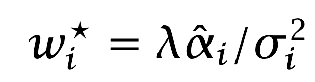
where λ is a positive constant chosen so that the portfolio meets a given budget constraint. What is the Sharpe ratio of the portfolio? The PnL is
The volatility of the portfolio is
The Sharpe is the ratio of the two.
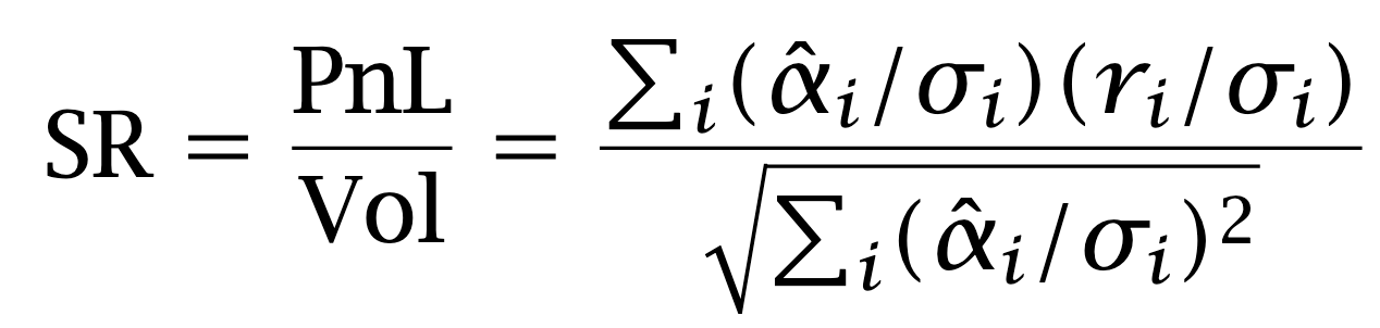
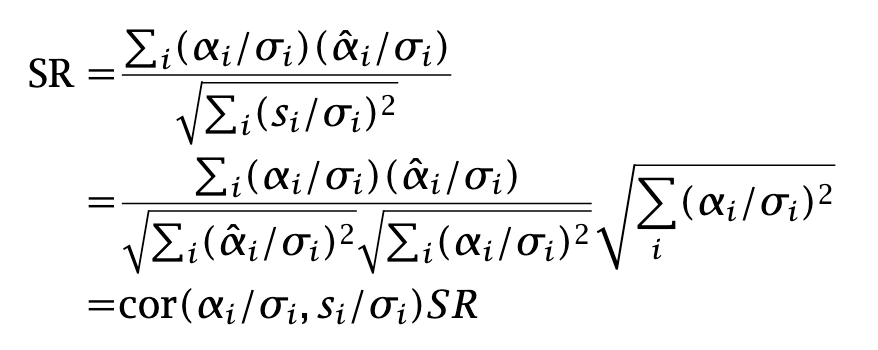
Almost there. Divide-and multiply-trick:
It is reasonable to assume that the sums in the numerator,
and
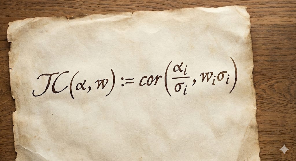
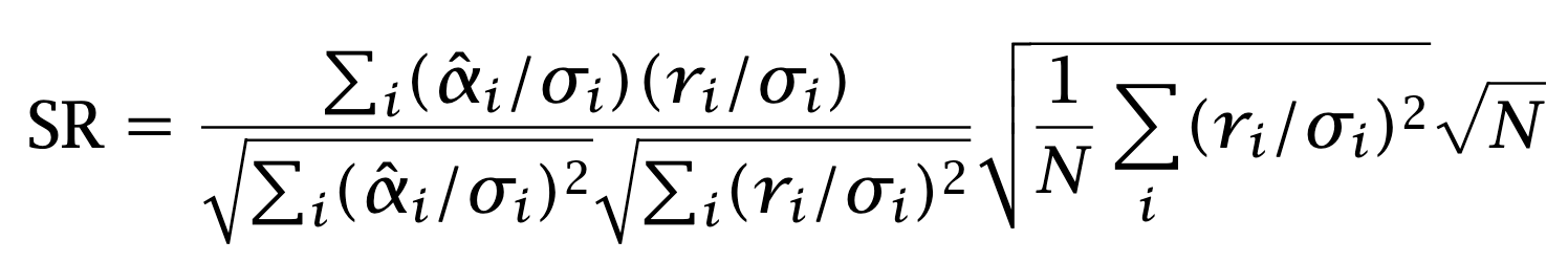
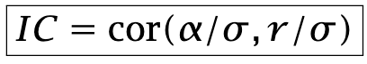
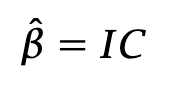
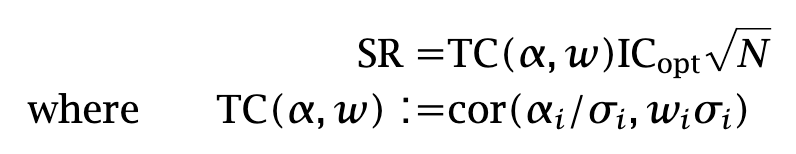
are zero, or very close to zero. Positive and negative positions should be approximately equal in number, and risk-adjusted net exposure should be approximately zero. The fraction can be interpreted as a correlation between risk-adjusted alphas and returns. Grinold calls this correlation the Information Coefficient:
It makes sense that the Sharpe ratio should be proportional to this coefficient. Consider the other factor in the formula. For large N, the average
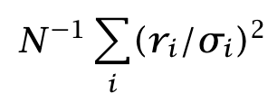
converges to one by the Law of Large Numbers. The formula for the Sharpe ratio therefore takes the form
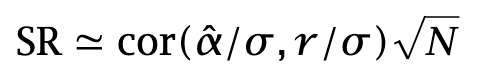
The Sharpe Ratio is the product of two factors. The first one is an intensive quantity. It does not depend on the number of assets. It is indicative of skills. The other one is an extensive quantity: it scales like the square root of the investment universe.
FLAM is intuitive and is useful in many ways. It points the attention to what really matters in cross-sectional alphas. If you have one-period out predictions for your cross-section, a research strategy suggested by FLAM is
Build a decent factor model to produce idiosyncratic returns and predicted volatilities.
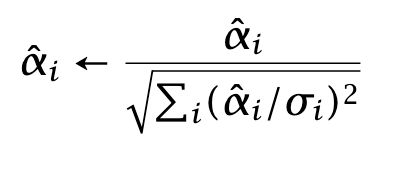
Generate predicted returns and rescale them:

Regress
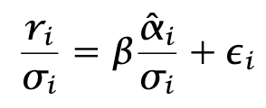
In this regression, the error terms εi have approximately unit variance. The formula for beta is
You have reduced your research program to the pursuit of two subproblems. The first is signal research, which I outlined above. The second is monetization: taking your alphas and turning them into a strategy that achieves a good real-life Sharpe ratio, despite execution costs, financing costs, and so on. This program, based on a separation of concerns, is followed to a large—though not universal—extent by most quantitative researchers. If we take a small step further, the signal research program can be generalized slightly:
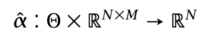
“Alphas” are a function from a parameter space Θ and a set of data Xt ∈ RNxM to RN. The data panel Xt contains M-dimensional vectors of features for each asset. This formulation encompasses an embarrassingly large array of choices, from simple linear combinations of columns to the latest and greatest learning architectures, with weights representable as a vector in Θ.

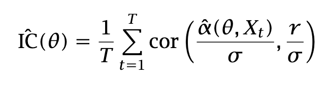
Compute the empirical IC each period, and average the IC:

Maximize the average IC , and/or compute its value over a ``covering’‘ of the parameter space Θ, i.e., θ1,…, θK. Compute a confidence interval using some methodology2.
Let us summarize what we assumed and what we did not assume, either explicitly or implicitly.
We assumed that:
Returns have finite variances (and therefore finite means).
Returns are temporally independent across periods.
Returns are identically distributed across periods.
Volatilities are known exactly.
Investors are mean–variance optimizers.
We did not assume that:
Predicted returns are accurate.
Returns are normally distributed.
Transfer Coefficient
Back to the process. We have signals alpha hat. Rewrite the expected PnL as
and let us write the Sharpe ratio:
We assumed that holdings were the solution of a mean–variance optimization, but in fact the relationship holds for general holdings wi:
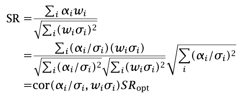
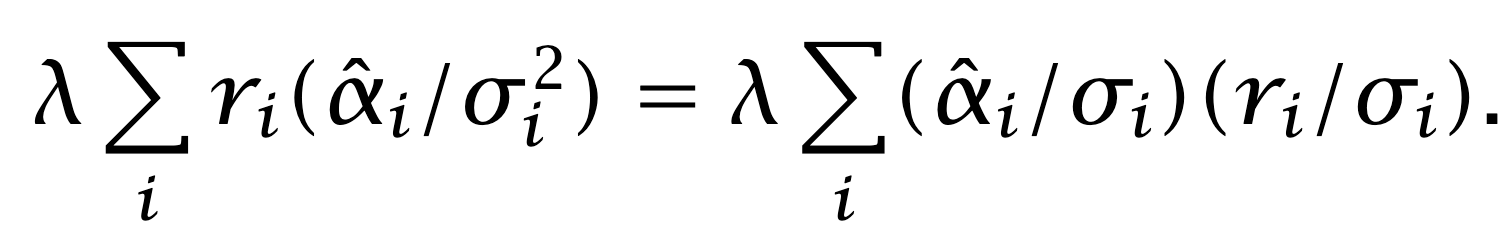
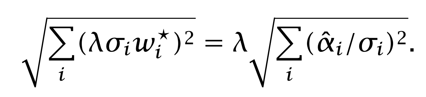
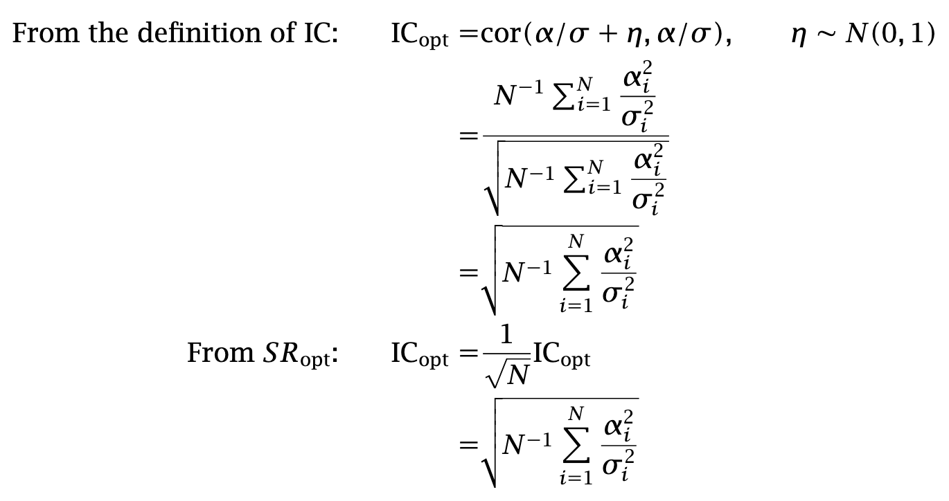
The quantity SRopt is the highest possible Sharpe ratio, achieved when forecasts are proportional to the true expected returns. We compute the corresponding ICopt in two ways:
Summing up, any Sharpe ratio is equal to
The Transfer Coefficient is always smaller than one. It represents the unavoidable degradation of the Sharpe ratio when we construct a portfolio under certain conditions, including:
Having inaccurate return predictions.
Having inaccurate volatility estimates.
Having accurate alpha and volatility predictions, yet constructing a portfolio that does not maximize Sharpe—either by solving a constrained Sharpe maximization problem or by not solving a Sharpe maximization problem at all.
There are two statements that this result does not imply. First, it does not follow that adding constraints always results in Sharpe degradation. In fact, when predictions are inaccurate, side constraints can ex ante improve the Sharpe ratio. As a simple example, consider an extreme case in which the investor has a grossly inaccurate set of volatility predictions. As a result, the sizing of optimal positions from mean–variance optimization is severely distorted. The optimizer may then choose to add a side constraint of the form ∑iwi2 ≤ L. verror in the volatilities. Secondly, it does say that
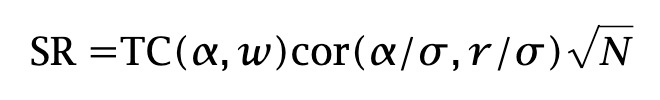
and not that
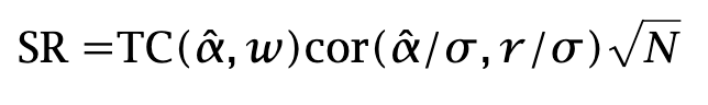
The “hat” makes all the difference. When return forecasts are inaccurate, the formula does not hold. Yet most people interpret the Transfer Coefficient as corresponding to the latter equation. The former equation is the one that actually holds, and because it requires knowledge of the true expected returns—which we cannot observe—most of its empirical utility vanishes.
In summary, we assumed that:
Returns have finite variances (and therefore finite means).
Returns are temporally independent across periods…
…and identically distributed in each period.
We know both the true expected returns and the volatilities of the assets.
We did not assume that:
Investors are mean–variance optimizers.
Returns are normally distributed.
What is to Be Done?
The original intent of the Transfer Coefficient is to establish a link between a pristine strategy and a strategy corrupted by the real world, as illustrated below:


This link, however, is not as solid as we once thought. What should we do? One approach is to compare the Sharpe ratios of the two strategies as if they were independent. For large T, the empirical Sharpe ratio is normally distributed. Asymptotically, under the null hypothesis that the Sharpe ratios are identical, the statistic
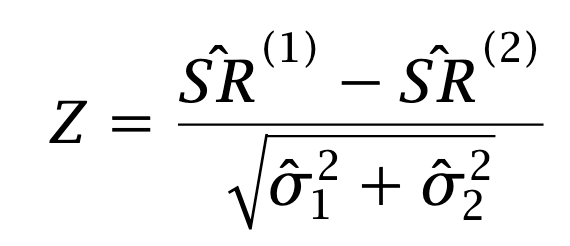
is distributed like a standard normal. The strategies, however, are not independent: their excess returns are paired. The correlation between the strategies is typically positive, and we can take advantage of that. The idea is to derive a statistic for the difference in Sharpe ratios under the assumption of paired observations. Such a statistic was derived by Jobson and Korkie in the large-sample asymptotic case3. The thrust of the paper is to compute a Taylor expansion of the statistic; the name for this technique is “delta method” and it is described in any asymptotic statistics textbook4. In The thrust of their paper is to compute a Taylor expansion of the statistic; the name for this technique is the delta method, and it is described in any asymptotic statistics textbook.
In applications, however, sample sizes are nowhere close to large. Many investors have observable track records of only one or two years of daily returns, and these returns are heavy-tailed. A bootstrap-based approach is therefore preferable. It is also much simpler than the analytical one. The steps are:
For i=1,…, B:
Resample with replacement the T pairs (r1,t, r2,t) into T pairs (r*1,t, r*2,t)
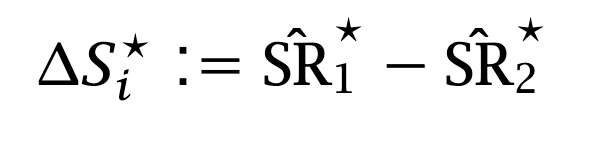
Compute the difference of the Sharpe Ratios from resampled data
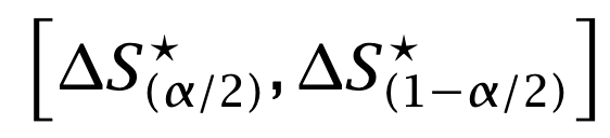
Compute the confidence interval from the empirical γ-quantile of the bootstrapped Sharpe differences.

And that’s it. Now you have a measure that includes uncertainty around the change in performance from signal to implementation.
As usual, I have created a pdf of this post, with more epsilon, deltas, and notably some details on Jobson-Korkie. And it prints nicely, if you need to.
Clarke, de Silva, Thorley. “The Fundamental Law of Active Portfolio Management”. J. Investment Management (2006), 4 (3), 54-72
I cover the subject in my book “The Elements of Quantitative Investing” (Wiley, 2025).
Jobson and Korkie, “Performance Hypothesis Testing with the Sharpe and Treynor Measures”. J. Finance (1981). 36, 889–908
See for example A. W. van der Vaart, “Asymptotic Statistics”. Cambridge University Press (2012)
Thanks, I'll never forget the difference between a pristine strategy and a real strategy now I have those contrasting images of Leonardo di Caprio.
And I'll check out the bootstrap approach, too.
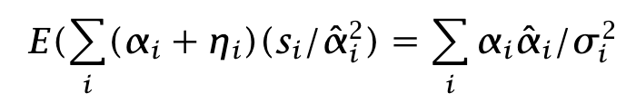
Nice paper. The equation 𝐸(∑(𝛼𝑖 + 𝜂𝑖)(𝑠𝑖/ ̂ 𝛼2𝑖 ) is a bit confusing(the one above equation 7), do you actually mean s / \sigma^2 instead of s/\alpha^2 ?