
On Timing Strategies
You thought it was hard. It is harder.


Dear portfolio manager: how many times have you received an email containing a sell-side research report highlighting the risk of a momentum crash? How many times have you read about factor seasonality? Or perhaps it is that month of the year when your competitors are underperforming, and you worry that they might reduce the size of your portfolio at the most inopportune time, dragging your PnL down with them. Every time you read these warnings or invitations, you wonder: should I take my volatility up? Down? Sideways (if such a thing is possible)?
These—and many others—are instances of timing signals in investing. They share a few common characteristics. First, there is some informative signal that makes us think a different performance of the strategy is more likely. Second, the signal, while informative, is noisy: there is a non-zero probability that it is wrong and that nothing changes. Lastly, these signals are infrequent. You can imagine a systematic strategy that trades several assets with time-varying expected returns. In that context, timing is not an overlay on the strategy; timing is the strategy.
Quite a lot rides on timing. First, the mental cycles of PMs. Second, the PnL of the portfolio. Third, some hedge funds even change their policies to take advantage of timing effects. If you truly believe that December and January are higher-Sharpe months for hedge funds, then it may make sense to anticipate the crystallization of bonuses to October, so that PMs are more risk-tolerant in January. This, too, is a form of timing.
I therefore thought it would be useful to have a simple model of timing exploitation. How do we quantify it? What should we do, ideally? And what is the benefit? The idea is to construct the simplest possible model of timing: just enough detail to be realistic, just enough parameters to be non-trivial, but concrete enough that they can be estimated. The model should be just within the reach of analytical treatment—or of an LLM, or a prolonged candidate interview.
The plan for this post is straightforward. I first describe the model and the optimal policy. Then I give some examples, followed by a discussion of the results. Finally, the proof and an example Google Sheet for playing with the numbers are provided as separate documents.
The Model
An investment strategy has two states: “Normal” or “Anomalous”, with Sharpe Ratios equal to SN and SA respectively.
We do not observe the state, but we have a signal y on the state of the strategy. The signal is random, iid, and takes two values: it is “Anomalous” with probability p and “Normal” with probability 1 - p. Given either signal value, the probability that the signal is accurately describing the true state is q.
Our objective is, given our noisy state signal, to deploy volatility over time so as to maximize the expected Sharpe ratio of the strategy. More precisely, we seek to identify a general policy: we allocate volatility x, given y with a probability distribution fy(x).
The Solution
The optimal strategy does not involve randomized volatility allocation. Instead, conditional on the signal, we allocate a deterministic level of volatility for that period. For Sharpe ratio optimization, the solution exhibits scale indeterminacy: if x(y) is Sharpe-optimal, then kx(y) is also optimal for any positive k. The optimal strategy is therefore characterized by the ratio of the optimal volatilities between the “anomalous” and “normal” states.
The optimal strategy does not depend on the frequency of the event. Define

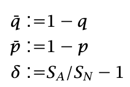
δ is the percentage change from normal to anomalous Sharpe. The optimal volatility ratio is
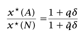
Example: if you think that SAS_ASA is 30% greater than SN next month, and you are right 80% of the time (not bad!), and you want to maximize the Sharpe ratio of your strategy (annual PnL divided by annual volatility), then you should scale up volatility by
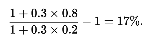
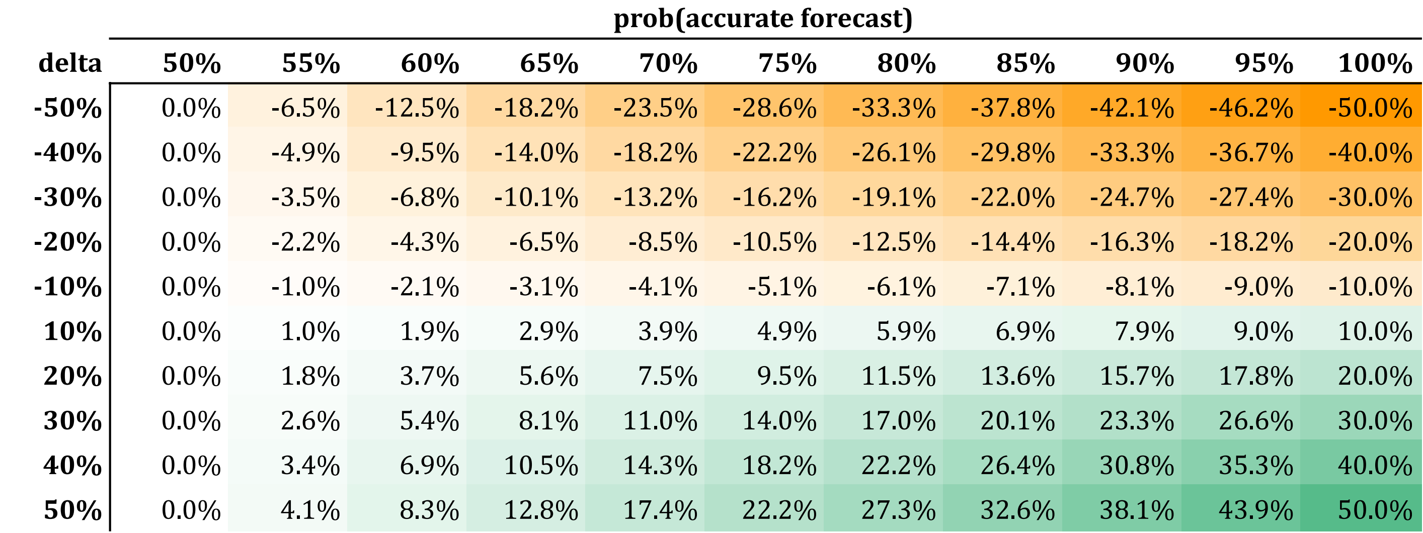
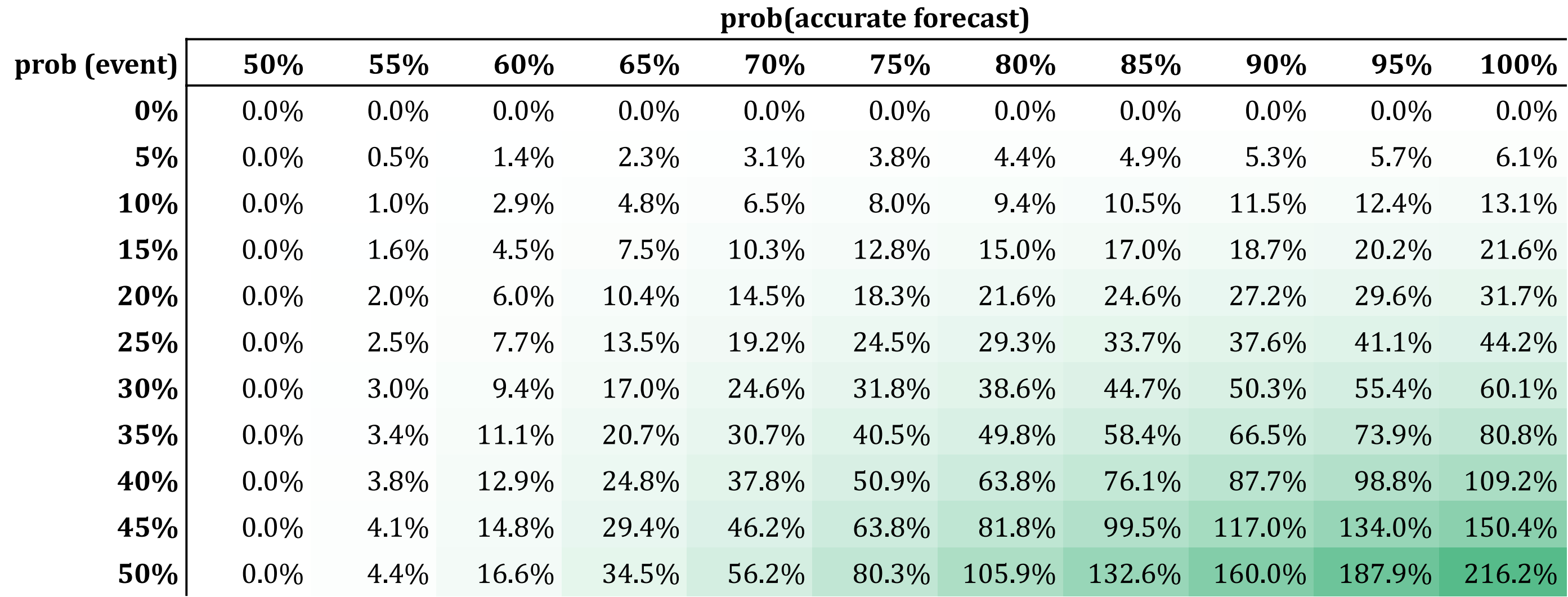
Do not increase it by 30%. As a first linear approximation (small δ), the percentage increase is (2q - 1)δ. Here is a table with optimal vol increases/decreases.
A small caveat. Suppose SA = -1 and SN = 1. Then δ = -2. And assume we have perfect foresight: q=1. Then the ratio of the optimal volatilities is -1. Of course: you know with certainty that the anomalous Sharpe is the opposite of the normal one, so you simply take the short position in the strategy. In other words, the correct interpretation of x* is that of a signed volatility.
The Sharpe ratio improvement, relative to the baseline of constant volatility, is
This also sense-checks, though it is less obvious. You need to have an edge in forecasting (q != 50%). This also sense-checks, though it is less obvious. You need to have an edge in forecasting Notice that if you are bad at forecasting, i.e., q < 0.5, , you are actually good at forecasting that an anomaly will not be present.
Example #1: Calendar Effects
There is weak evidence of hedge fund annual outperformance in certain months, primarily December and January. This, in turn, has led hedge funds to encourage portfolio managers to increase deployed volatility during those periods. The periodic outperformance of hedge funds has even led some firms to change the calendar used for bonus calculations. This seems like a clever thing to do, but I am not aware of any explicit analysis of the associated costs and benefits. Changing the calendar is a complicated undertaking—unless you are Santa, in which case it is impossible. Your livelihood depends on it.
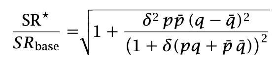
Consider first a scenario in which December and January have a Sharpe ratio that is 20% higher than in other months. The resulting improvement in the average Sharpe ratio is shown below. Assuming that about 20% of months exhibit outperformance and that forecasting accuracy is perfect (q=100%), the percentage improvement in the average Sharpe ratio relative to a constant-volatility allocation is very modest: about 0.3%.
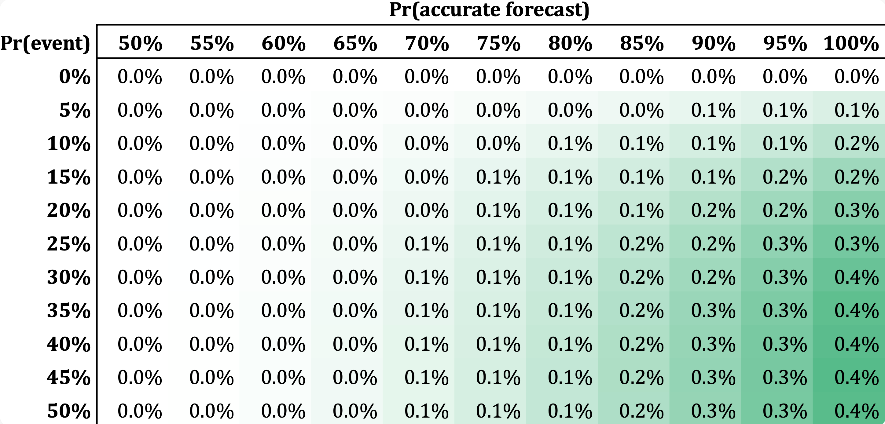
But consider a more pronounced scenario, with a 50% outperformance in the anomalous-Sharpe regime. In this case, the improvement is larger, but still quite small: 1.6%.
Example #2: Factor Timing
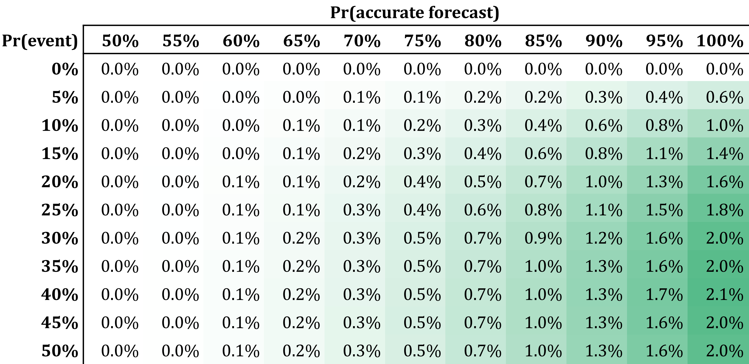
A similar, but distinct, example is one in which we receive an out- or underperformance signal for a factor. For instance, we may have an indicator of a possible degradation. These signals are low frequency and can imply large deviations from the expected Sharpe ratio of the factor. We consider the case p=10% with the anomalous Sharpe ranging from -50% to 50%. The table below shows the results for several levels of forecast accuracy. In this case as well, we find that the benefits from timing are modest, peaking at about 1.2%.
Example #3: Derisking & Crashes
Certain strategies are prone to crashes. There are also indicators that can alert decision-makers that, with a given probability, a strategy may experience a large negative Sharpe ratio. Below, I show the Sharpe improvements for a case in which the anomalous Sharpe is equal to −50% of the base Sharpe. It is worth noting that, while rare (e.g., p ~ 5%), these events can be anticipated with relatively high precision (e.g., q ~ 80%). In this case, the Sharpe ratio improvement is on the order of 4-5%.
Discussion
The examples I provided resemble realistic scenarios. They show that, even with complete forecasting accuracy (q=100%q = 100\%q=100%), the impact of optimal timing on the Sharpe ratio is moderate.
In our modeling, I ignored the transaction costs associated with scaling the portfolio up and down. Their impact would further reduce the benefits of scaling. The scaling factor itself can be large: for a 50% increase or decrease in Sharpe, the optimal increase or decrease in position size is approximately 30%.
I also considered only Sharpe ratio maximization. This is reasonable for recurring, non-existential opportunities and threats. If you can destroy the Bank of England, or a meteorite can destroy you, do not use these prescriptions.
Love this approach. But when you develop the strategy in the first place - don't your have priors regarding why it generates (hopefully positive) returns, and under which conditions those returns occur. Shouldn't those logical insights inform whether (if/when) a timing strategy would work?
As a semi-systematic macro investor, I can often look at backtests or hear pitches and deduce which market environments a strategy generates most of its returns under (e.g. early cycle, hiking cycles..). To me, it's a critical thought experiment, because if you have the right macro quant tools to test these deductions and they're right, you can construct hedges (e.g. strategies that perform in different macro environments) or overlays (e.g. only run this strategy early cycle) to 'time' the strategy.
If someone can't predict/explain when, not just why, a strategy generates its performance - I have less confidence in its out-of-sample performance.
I'm curious how the model scales for idiosyncratic events like earnings sentiment. In that case we know the event timing, and the Sharpe delta is likely massive. Since the approximation assumes small delta, would the exact solution suggest much more aggressive sizing for these high conviction moments or does the signal noise around earnings still wash out the benefits?